Tutorial
This tutorial will take the user through the basics of atomic data needed for Collisional Radiative (CR) modeling. The python scripts for these examples can be found in the ‘examples’ folder.
For a detailed introduction to CR theory see the ColRadPy paper included in the ‘user_doc’ folder. Summers 2006 also provides a more detailed overview of CR theory.
Neither the local thermodynamic equilibrium (LTE) or conornal approximations are valid for fusion plasmas. These plasmas must be modeled with a collisional radiative (CR) model which includes effects of electron density. Collisional Radiative theory has been updated to included general collisional radiative (GCR) theory, this is outlined in (Summers 2006).
The tutrial will go over the following major topics
Installing ColRadPy Installing ColRadPy
The atomic data input for colradpy is overviewed in Atomic Data and the ADF04 File
Running ColRadPy will be outlined in Running ColRadPy
Built in post processes in ColRadPy is described in Post processing analysis built in functions
Posted processing for advanced users will be outlined in Post processing analysis advanced
The generalized collisional radiative coefficients will be discussed in Generalized radiative coefficients (GCRs)
Functionality for advanced users is outlined in Advanced functionality
Ionization balance is outlined in Ionization Balance
Installing ColRadPy
ColRadPy should work with any python 3.6 distribution. However, ColRadPy is only tested with the anaconda distribution of python 3.6. ColRadPy requires numpy, matplotlib, re, scipy, sys, collections packages. For local installation of ColRadPy In the ‘colradpy’ directory.
1python setup.py build
2python setup.py install
Colradpy can now be called like anyother package.
1from colradpy import colradpy #import the colradpy class
2from colradpy import ionization_balance #import the ionization_balance class
Atomic Data and the ADF04 File
Atomic data is generally made by calculating cross-sections (probablity) of transitions. From these cross-sections rates are then made by convolving with a maxwellian temperature distriubtion (or some of distribution) of electron energies with the cross section. The rates produced by this method are what is used in the CR model.
The ADF04 file format from ADAS that is used to hold atomic rate data for input into the CR model.
Electron Impact De/Excitation
Electron impact excitation and deexcitation is what causes transitions be the ground and excited states and within excited states. There rates are stored as “effective collisional strengths” in the adf04 file. These can then be converted to the excitiation and deexcitation rates that are needed for CR modeling.
Electron Impact Ionization
Electrons can also ionize atoms to the next charge state. Ionization can be stored in the adf04 file as reduced ionization rates. ColRadPy is also capable of making ECIP ionization rates. ECIP ionization is a very approximate way of making ionization and should be avoid if possible. Ground and metastable states generally have calculated ionization rates while excited states generally have rates that are supplimented with ECIP.
Radative Recombination
Dielectronic Recombination
Dielectronic recombination is the dominant recombination process in many plasmas. Dielectronic recombination is a two step process. First, there is a resonance capture of a free electron. In this processes a bound electron gains some energy and the free electron loses some energy. Second, the atom radiates a phonton.
Three-Body Recombination
Three-body recombination is calculated from using detailed balance from the ionization. In this process, free electrons and a ion recombine to produce a new ion and one free electron.
Solutions
Once rates from the basic atomic data have been input. ColRadPy can then solve the set of rate equations known as the collisional radiative equations. There are two ways that ColRadPy can solve the CR set of equations. The general user will probably be interested in the first way of solving the CR equations, this is same way ADAS solves the equations. The Quasistatic approximation solves the equations assuming that excited states do not have time changing populations. It assumes that these populations and in their equilbrium values with the ground and any metastable levels. This is the way that ADAS solves the CR set of equations.
ColRadPy is also capable of solving the system of equations time dependently using the matrix exponentialation method. This solution makes no assumptions of equilbrium time scales for excited states. This is an excact solution. In equilbrium, the non-quasistatic and quastistic solutions will be the same.
Running ColRadPy
ColRadPy requires multiple inputs from the user to run. The basic quasistatic run will be discussed first. This should be sufficient for most users. Once the code runs data is store in a dictionary accessed through the ‘.data’ method. The entries of this dictionary and descriptions are documented here.
Atomic data input file - currently this is limitted to an ADF04 file but there is nothing special about it.
array of metastable levels - This is an array of levels that includes the ground and any levels that could be considered metastable.
temperature grid - This is an array of electron temperatures for the calculation in eV.
Density grid - This is an array of electron densities for the calculation in cm-3.
In this example Be II (Be+) is used because it is a simple system that has a parent ion (the next charge state) that has a metastable. This allows all of the different functionality to be shown and tested.
The module must be executed
Input file, temperature, density and metastable inputs defined.
Ionization, recombination options chosen default values are true
There are are highlevel class definitions that a general user can use. These high level definitions will be shown as well as the more basic definitions that these high level definitions call. A basic user needs to only care about the high level definitions
Below is an example of running ColRadPy. The user chooses an input adf04 file, temperature and density grids as well as the number of metastables. If you don’t know how many metastables exist only choose level ‘0’ (the ground) as being metastable. Choices were also made to include ionization and recombination. Note that metastable levels are only important if the plasma is not in equilbrium. In equilbrium metastable fraction is set and will not vary for a given temperature and density.
The ‘use_recombination’ flag when true will use any recombination rates that are included in the adf04 file.
The ‘use_recombination_three_body’ flag when true will have ColRadPy make and include three body recombination rates.
Note inorder to have three body recombination there must be some ionization included in the calculation.
The ‘use_ionization’ flag when true will use any ionization rates that are included in the adf04 file.
The ‘suppliment_with_ecip’ when true will have ColRadPy make ECIP ionization rates and include these rates anywhere that there are no ionization rates included in the adf04 file.
Note that ionization should always be included in the calculation even if it is just ECIP. Ionization can significantly change both absolute values of PECs as well as relative values of PECs.
 1 import sys
 2 sys.path.append('../') #starting in 'examples' so need to go up one
 3 from colradpy_class import colradpy
 4 import numpy as np
 5
 6 fil = 'cpb03_ls#be0.dat' #adf04 file
 7 temperature_arr = np.linspace(1,100,100) #eV
 8 metastable_levels = np.array([0])   #metastable level, just ground chosen here
 9 density_arr =     np.array([1.e13,4.e14]) # cm-3
10
11 #calling the colradpy class with the various inputs
12 be = colradpy(fil,metastable_levels,temperature_arr,density_arr,use_recombination=True,
13               use_recombination_three_body = True,use_ionization=True,suppliment_with_ecip=True)
14
15 be.solve_cr() #solve the CR equations with the quasistatic method
‘be’ is now a colradpy class that has been solved. There are various methods for getting the data out. Data that required ColRadPy to solve the CR set of equations is now stored in the ‘processed’ sub dictionary. There are many different calls that could be made from the class documented here.
--- Show/details of solve_cr()---Data from the calculation is now avaible in the ‘.data’ dictionary. Various postpocessing can be done to now analysis the calcuation.
Post processing analysis built in functions
There are some built in functions avaible for post processing analysis these will of use for the general user. The basic functions require minimal knowelge of the underlying datastructure. These basic functions will be overviewed first then a more complex analysis will be presented after.
The theorical spectrum can be plotted describe in Plotting Theorical Spectrum (PEC sticks)
The line ratios versus temperature and density is describe in Plotting PEC ratios
Plotting Theorical Spectrum (PEC sticks)
The theorical spectral spectrum from the adf04 file can be plotted with the below command. The parameters are the lists or arrays of the index of the metastable, temperature and density grids. WARNING Note that wavelengths will not match NIST wavelengths unless the adf04 energy levels have been shifted to the NIST values. This generally hasn’t been done in the past so there are many adf04 files that don’t use NIST energy values.
1 be.plot_pec_sticks([0],[0],[0])
Plotting PEC ratios
Spectral line intenties are functions of both electron temperature and density as well as ion density. Different spectral lines will have different functional forms on temperature and density. It is therefore possible to find ratios of spectral lines that are depenended on either temperature or density as the ion density cancels out. It is then possible to dianose electron temperature and density from line ratios where the charge state exists in the plasma.
Temperature ratios can be plotted with the below function. The temperature ratio of the two pecs will be plotted with new figures made for each density and metastable requested. The inputs are the indexes of pec1, pec2, array of densities and array of metastables
1 be.plot_pec_ratio_temp(0,1,[0],[0])
1 be.plot_pec_ratio_dens([0],[0],[0])
Post processing analysis advanced
Photon emissivity coefficients (PECs)
A theortical spectrum can be made from the PEC coefficients. PEC coefficient are stored in array that has shape (#pecs,metastable,temperature,density). The code below produces a PEC spectrum for on temperature and density. The wavelength and pec arrays share the same length.
 1import matplotlib.pyplot as plt
 2plt.ion()
 3met = 0 #metastable 0, this corresponds to the ground state
 4te = 0 #first temperature in the grid
 5ne = 0 #frist density in the grid
 6
 7fig, ax1 = plt.subplots(1,1,figsize=(16/3.,9/3.),dpi=300)
 8fig.subplots_adjust(bottom=0.15,top=0.92,left=0.105,right=0.965)
 9ax1.vlines(be.data['processed']['wave_air'],
10           np.zeros_like(be.data['processed']['wave_air']),
11           be.data['processed']['pecs'][:,met,te,ne])
12ax1.set_xlim(0,1000)
13ax1.set_title('PEC spectrum  T$_e$=' +str(be.data['user']['temp_grid'][te])+\
14              ' eV  ne=' + "%0.*e"%(2,be.data['user']['dens_grid'][ne]) + ' cm$^{-3}$',size=10)
15ax1.set_xlabel('Wavelength (nm)')
16ax1.set_ylabel('PEC (ph cm$^{-3}$ s$^{-1}$)')

Often the index of a specific pec is wanted to find its temperature or density dependence. This can be accomplished in two basic ways.
Upper and lower levels of the transitions are known
The wavelength of the transition is known
There is a map from transition numbers to pec index levels. .data[‘processed’][‘pec_levels’] has the same order as .data[‘processed’][‘wave_air’] and .data[‘processed’][‘pecs’].
 1print(np.shape(be.data['processed']['wave_air']),
 2      np.shape(be.data['processed']['pecs']),
 3      np.shape(be.data['processed']['pec_levels']))
 4#(320,) (320, 3, 1, 1) (320, 2)
 5
 6upper_ind = 7 #ninth excited state
 7lower_ind = 0  #ground state
 8
 9pec_ind = np.where( (be.data['processed']['pec_levels'][:,0] == upper_ind) &\
10                    (be.data['processed']['pec_levels'][:,1] == lower_ind))[0]
11
12#plot the temeprature dependence of the chosen pec at first density in the grid
13fig, ax1 = plt.subplots(1,1,figsize=(16/3.,9/3.),dpi=300)
14fig.subplots_adjust(bottom=0.15,top=0.93,left=0.105,right=0.965)
15ax1.set_title('Temperature dependence of line ' +\
16              str(be.data['processed']['wave_air'][pec_ind]) +' nm',size=10)
17ax1.plot(be.data['user']['temp_grid'],be.data['processed']['pecs'][pec_ind[0],met,:,ne])
18ax1.set_xlabel('Temperature (eV)')
19ax1.set_ylabel('PEC (ph cm$^{-3}$ s$^{-1}$)')
20
21#plot the density dependence of the chosen pec at first density in the grid
22fig, ax1 = plt.subplots(1,1,figsize=(16/3.,9/3.),dpi=300)
23fig.subplots_adjust(bottom=0.15,top=0.93,left=0.125,right=0.965)
24ax1.set_title('Density dependence of line ' +\
25              str(be.data['processed']['wave_air'][pec_ind]) +' nm',size=10)
26ax1.plot(be.data['user']['dens_grid'],be.data['processed']['pecs'][pec_ind[0],met,te,:])
27ax1.set_xlabel('Density (cm$^{-3}$)')
28ax1.set_ylabel('PEC (ph cm$^{-3}$ s$^{-1}$)')
If the wavelength of a line of interest is known, the index can be found by looking at the wavelength array. The indices of all pecs that fall within the upper and lower bound of the ‘where’ statement are returned. PECs can generally be distinguished by the actual value, large lines that are of interest have much large PEC values, this can allow


1#want to find the index of Be I line at 351.55
2pec_ind = np.where( (be.data['processed']['wave_air'] <352) &\
3                    (be.data['processed']['wave_air'] >351))
4print('Wavelength from file ' + str(be.data['processed']['wave_air'][pec_ind[0]]))
5#Wavelength from file [351.55028742]
6print('PEC upper and lower levels '+ str(be.data['processed']['pec_levels'][pec_ind[0]]))
7#PEC upper and lower levels [[25  2]]
Generalized radiative coefficients (GCRs)
The generalized collsional radiative coefficients are calculated by ColRadPy as well. A description of these can be found in (Summers 2006), (Johnson 2019). GCR coefficients are often used as inputs to plasma transport codes. GCR coefficients are also used as inputs to ionization balance calculations which will be discussed later. This allows for different ionization stages to be linked.
For example, the total ionization from one charge state to the other is defined as the SCD. The total recombination from a charge state to the charge state of interest is defined as the ACD. This gives the rate of population transfer from one ionization state to a lower ionization state. The situation for systems with metastable states requires that the effective ionization and recombination rates be metastable resolved. In addition, it requires metastable cross coupling coefficients known as QCD and XCD coefficients.
Generally it is of interest to look at how the GCR coefficients change with some parameter such as temperature. Plots are shown below of the different GCRs.
A physical description of the GCRs can be helpful in interpreting the meaning behind them.
Metastable Cross Coupling Coefficient (QCD)
The QCD coefficient represents the transfer of population from one metastable state to another within the ionization state of interest and includes both direct population transfer between metastable states as well as the transfer via an intermediate excited state.
GCR Ionization Coefficient (SCD)
The total ionization from one charge state to the other is defined as the SCD.
GCR Recombination Coefficient (ACD)
The total recombination from a charge state to the charge state of interest is defined as the ACD.
Metastable Parent Cross Coupling Coefficient (XCD)
The XCD coefficient represents the transfer of population between metastable states from the ionization stage just above the stage of interest. Populations in the upper ionization stage can recombine into the ionization state of interest from one metastable, redistribute through all the states and then ionize back into a different metastable state of the upper ionization state.
GCR Examples
For this example we will look at Be II this is soley because Be III has two metastable states. This means that the XCD will have non-zero values. Remeber the call from before for Be I.
 1import sys
 2sys.path.append('../')
 3from colradpy_class import colradpy
 4import numpy as np
 5
 6fil = 'cpb03_ls#be1.dat' #adf04 file
 7temperature_arr = np.linspace(1,100,20) #eV
 8metastable_levels = np.array([0,1])   #ground and level 1 chosen to be metastable
 9density_arr =     np.array([1.e13,8.e13,4.e14]) # cm-3
10beii = colradpy(fil,metastable_levels,temperature_arr,density_arr,use_recombination=True,
11              use_recombination_three_body = True,use_ionization=True,suppliment_with_ecip=True)
12beii.solve_cr()
 1#plotting the QCD
 2import matplotlib.pyplot as plt
 3plt.ion
 4fig, ax1 = plt.subplots(1,1,figsize=(16/3.,9/3.),dpi=300)
 5fig.subplots_adjust(bottom=0.15,top=0.92,left=0.125,right=0.965)
 6ax1.plot(beii.data['user']['temp_grid'],
 7         beii.data['processed']['qcd'][0,1,:,0]*1e5,
 8         label = 'metastable cross coupling coefficient 1->2')
 9
10ax1.plot(beii.data['user']['temp_grid'],
11         beii.data['processed']['qcd'][1,0,:,0]*1e5,
12         label = 'metastable cross coupling coefficient 2->1')
13ax1.legend()
14ax1.set_title('QCD plot')
15ax1.set_xlabel('Temperature (eV)')
16ax1.set_ylabel('QCD * 10$^5$ (cm$^{-3}$ s$^{-1}$)')

 1#plotting the SCD
 2fig, ax1 = plt.subplots(1,1,figsize=(16/3.,9/3.),dpi=300)
 3fig.subplots_adjust(bottom=0.15,top=0.92,left=0.125,right=0.965)
 4ax1.plot(beii.data['user']['temp_grid'],
 5         beii.data['processed']['scd'][0,0,:,0],
 6         label = 'metastable cross coupling coefficient 1->1+')
 7
 8ax1.plot(beii.data['user']['temp_grid'],
 9         beii.data['processed']['scd'][0,1,:,0],
10         label = 'metastable cross coupling coefficient 1->2+')
11
12ax1.plot(beii.data['user']['temp_grid'],
13         beii.data['processed']['scd'][1,0,:,0],
14         label = 'metastable cross coupling coefficient 2->1+')
15
16ax1.plot(beii.data['user']['temp_grid'],
17         beii.data['processed']['scd'][1,1,:,0],
18         label = 'metastable cross coupling coefficient 2->2+')
19
20ax1.legend(fontsize='x-small',loc='best')
21ax1.set_title('SCD plot')
22ax1.set_xlabel('Temperature (eV)')
23ax1.set_ylabel('SCD (ion cm$^{-3}$ s$^{-1}$)')

 1#plotting the ACD
 2fig, ax1 = plt.subplots(1,1,figsize=(16/3.,9/3.),dpi=300)
 3fig.subplots_adjust(bottom=0.15,top=0.92,left=0.075,right=0.965)
 4ax1.plot(beii.data['user']['temp_grid'],
 5         beii.data['processed']['acd'][0,0,:,0],
 6         label = 'metastable cross coupling coefficient 1+->1')
 7
 8ax1.plot(beii.data['user']['temp_grid'],
 9         beii.data['processed']['acd'][0,1,:,0],
10         label = 'metastable cross coupling coefficient 2+->1')
11
12ax1.plot(beii.data['user']['temp_grid'],
13         beii.data['processed']['acd'][1,0,:,0],
14         label = 'metastable cross coupling coefficient 1+->2')
15
16ax1.plot(beii.data['user']['temp_grid'],
17         beii.data['processed']['acd'][1,1,:,0],
18         label = 'metastable cross coupling coefficient 2+->2')
19
20ax1.legend(fontsize='x-small',loc='best')
21ax1.set_title('ACD plot')
22ax1.set_xlabel('Temperature (eV)')
23ax1.set_ylabel('ACD (rec cm$^{-3}$ s$^{-1}$)')

 1#plotting the XCD
 2fig, ax1 = plt.subplots(1,1,figsize=(16/3.,9/3.),dpi=300)
 3fig.subplots_adjust(bottom=0.15,top=0.92,left=0.12,right=0.965)
 4ax1.plot(beii.data['user']['temp_grid'],
 5         beii.data['processed']['xcd'][0,1,:,0],
 6         label = 'metastable cross coupling coefficient 1+->2+')
 7
 8ax1.plot(beii.data['user']['temp_grid'],
 9         beii.data['processed']['scd'][1,0,:,0],
10         label = 'metastable cross coupling coefficient 2+->1+')
11ax1.legend(fontsize='x-small',loc='best')
12ax1.set_title('XCD plot')
13ax1.set_xlabel('Temperature (eV)')
14ax1.set_ylabel('XCD (cm$^{-3}$ s$^{-1}$)')

Determining Populating Mechanisms
One feature unique to ColRadPy is the ability to determine the populating mechanism of levels. This allows one to see which levels in a calculation are important to modeling the spectral lines of interest. This allows those that generate the atomic data to know which transitions are required to accurately model spectral lines. With this new analysis technique, it is possible to identify transitions that are the most important and allow for complex systems such as high-Z near neutral systems to be simplified.
ColRadPy also allows the user to determine which intermediate levels populate a level of interest withThis is don if the summation is not carried out from the calculation of the QCD. This allows one to see which levels in a calculation are important to modeling the spectral lines of interest.
 1#plotting the populating levels
 2plt.figure()
 3plt.figure();plt.plot(be.data['processed']['pop_lvl'][0,:,0,0,0]/\
 4                      np.sum(be.data['processed']['pop_lvl'][0,:,0,0,0]))
 5
 6plt.figure();plt.plot(be.data['processed']['pop_lvl'][0,:,0,10,0]/\
 7                      np.sum(be.data['processed']['pop_lvl'][0,:,0,10,0]))
 8
 9plt.figure();plt.plot(be.data['processed']['pop_lvl'][0,:,0,-1,0]/\
10                      np.sum(be.data['processed']['pop_lvl'][0,:,0,-1,0]))
11
12plt.legend()
13plt.xlabel('Level number (#)')
14plt.ylabel('Populating fraction (-)')
15
16#plotting the populating fraction from the ground versus temperature
17plt.figure()
18plt.plot(be.data['user']['temp_grid'],
19          be.data['processed']['pop_lvl'][10,0,0,:,0]/\
20          np.sum(be.data['processed']['pop_lvl'][10,:,0,:,0],axis=0))
21
22plt.xlabel('Temperature (eV)')
23plt.ylabel('Populating fraction from ground (-)')

This shows that as temperature increase other excited levels contributed more and more to the first excited state

This shows that as the temperature increases the ground tributes less to the total population of level 1.
Advanced functionality
Time dependent CR modeling
ColRadPy is also capable of solving the full collisional radiative matrix time-dependently. This can be important for systems where there is significant population in many excited states or where ultra fast timescales need to be considered. Instead of the quasi-static approximation used in Equation 4 where excited states are assumed to have no population change, the matrix is solved as a system of ordinary differential equations n (t) = An(t). This method used to solve the system of equations was adapted from R. LeVeque.
Case in which with and without a source term can be considered in ColRadPy. The case without a source term can used in a system like a linear machine with views that are transverse to the direction of motion of the particles.
A source term can be used when the line of sight includes a source of particles. The source term could also be used to model the pumping of specific levels with LIF.
 1import sys
 2sys.path.append('../')
 3from colradpy_class import colradpy
 4import numpy as np
 5import matplotlib.pyplot as plt
 6
 7#Time dependent CR modeling
 8td_t = np.geomspace(1.e-5,.1,1000)
 9td_n0 = np.zeros(30)
10td_n0[0] = 1.
11
12fil = 'cpb03_ls#be0.dat' #adf04 file
13temperature_arr = np.array([10]) #eV
14metastable_levels = np.array([0])   #metastable level, just ground chosen here
15density_arr =     np.array([1.e9]) # cm-3
16be = colradpy(fil,metastable_levels,temperature_arr,density_arr,use_recombination=True,
17              use_recombination_three_body = True,use_ionization=True,suppliment_with_ecip=True,
18              td_t=td_t,td_n0=td_n0,td_source=td_s)
19be.solve_cr()
20be.solve_time_dependent()
21
22fig, ax1 = plt.subplots(1,1,figsize=(16/3.,9/3.),dpi=300)
23fig.subplots_adjust(bottom=0.15,top=0.92,left=0.1,right=0.965)
24plt.plot(be.data['user']['td_t'],
25         be.data['processed']['td']['td_pop'][0,:,0,0],
26         label='Ground')
27plt.plot(be.data['user']['td_t'],
28         be.data['processed']['td']['td_pop'][1,:,0,0],
29         label='level 1')
30plt.plot(be.data['user']['td_t'],
31         be.data['processed']['td']['td_pop'][-1,:,0,0],
32         label='ion')
33ax1.legend(fontsize='x-small',loc='best')
34ax1.set_title('Time dependent solution of CR Be I no source term')
35ax1.set_xlabel('Time (s)')
36ax1.set_ylabel('Population (-)')

This time dependent collisional radiative model shows the time history for all Be I levels and the ground sate of Be II. This is the non-quasistatic solution, for a light system like Be the which only has one metastable the quasistatic approximation and non-quastatic solutions will give similiar results it is only for heavy species such as Mo and W where the quasistatic approximation starts to break down that this non-quasistatic solution is required.
 1td_t = np.geomspace(1.e-5,1,1000)
 2td_n0 = np.zeros(30)
 3td_n0[0] = 1.
 4td_s = np.zeros(30)
 5td_s[0] = 1.
 6fil = 'cpb03_ls#be0.dat' #adf04 file
 7temperature_arr = np.array([10]) #eV
 8metastable_levels = np.array([0])   #metastable level, just ground chosen here
 9density_arr =     np.array([1.e8]) # cm-3
10be = colradpy(fil,metastable_levels,temperature_arr,density_arr,use_recombination=True,
11              use_recombination_three_body = True,use_ionization=True,suppliment_with_ecip=True,
12              td_t=td_t,td_n0=td_n0,td_source=td_s)
13
14be.solve_cr()
15be.solve_time_dependent()
16
17fig, ax1 = plt.subplots(1,1,figsize=(16/3.,9/3.),dpi=300)
18fig.subplots_adjust(bottom=0.15,top=0.92,left=0.115,right=0.965)
19plt.plot(be.data['user']['td_t'],
20         be.data['processed']['td']['td_pop'][0,:,0,0],
21         label='Ground')
22plt.plot(be.data['user']['td_t'],
23         be.data['processed']['td']['td_pop'][1,:,0,0],
24         label='level 1')
25plt.plot(be.data['user']['td_t'],
26         be.data['processed']['td']['td_pop'][-1,:,0,0],
27         label='ion')
28ax1.legend(fontsize='x-small',loc='best')
29ax1.set_title('Time dependent solution of CR Be I with source term')
30ax1.set_xlabel('Time (s)')
31ax1.set_ylabel('Population (-)')

Time dependent solution with a constant source term of particles in the ground state. This could be used to model spectra where there is a constant erosion term from the wall. This could also be use to model level pumping in LIF systems.
Split LS resolved data to LSJ
ColRadPy is able to split PECs from term resolved (LS) into level resolved (LSJ) values. This currently does put PECs at the NIST wavelengths, a user must do this manually for now. In the future this will be done automatically using the NIST database.
 1import sys
 2sys.path.append('../')
 3from colradpy_class import *
 4import numpy as np
 5
 6he = colradpy('./mom97_ls#he1.dat',[0],np.array([20]),np.array([1.e13]),use_recombination=False,
 7               use_recombination_three_body = False,use_ionization=True)
 8
 9he.solve_cr()
10he.split_pec_multiplet()
11
12wave_8_3 = np.array([468.5376849,468.5757974,468.5704380])
13ind_8_3 = np.where( (he.data['processed']['pec_levels'][:,0] == 8) & \
14                    (he.data['processed']['pec_levels'][:,1] == 3))[0]
15
16wave_6_5 = np.array([468.5407225,468.5568006])
17ind_6_5 = np.where( (he.data['processed']['pec_levels'][:,0] == 6) & \
18                   (he.data['processed']['pec_levels'][:,1] == 5))[0]
19
20wave_7_3 = np.array([468.5524404,468.5905553])
21ind_7_3 = np.where( (he.data['processed']['pec_levels'][:,0] == 7) & \
22                    (he.data['processed']['pec_levels'][:,1] == 3))[0]
23
24wave_9_4 = np.array([468.5703849, 468.5830890, 468.5804092])
25ind_9_4 = np.where( (he.data['processed']['pec_levels'][:,0] == 9) & \
26                    (he.data['processed']['pec_levels'][:,1] == 4))[0]
27
28wave_6_4 = np.array([ 468.5917884, 468.5757080, 468.5884123])
29ind_6_4 = np.where( (he.data['processed']['pec_levels'][:,0] == 6) & \
30                    (he.data['processed']['pec_levels'][:,1] == 4))[0]
31
32
33wave_468 = np.hstack((wave_8_3,wave_6_5,wave_7_3,wave_9_4,wave_6_4))
34pecs_468 = np.vstack((he.data['processed']['split']['pecs'][ind_8_3[0]],
35                      he.data['processed']['split']['pecs'][ind_6_5[0]],
36                      he.data['processed']['split']['pecs'][ind_7_3[0]],
37                      he.data['processed']['split']['pecs'][ind_9_4[0]],
38                      he.data['processed']['split']['pecs'][ind_6_4[0]]))[np.argsort(wave_468)]
39wave_468 = wave_468[np.argsort(wave_468)]
40
41
42
43plt.figure()
44plt.vlines(wave_468,np.zeros_like(wave_468),pecs_468[:,0,0,0])
Ionization Balance
An ionization balance can be used to get the relative abundances of charge states in a given species. The relative populations of charge states are solved using the GCR coefficient that are calculated from the CR set of equations. A matrix similiar to the CR matrix is assembled using the GCR rate coefficients. The QCD rates transfer population between metastable states in one ionization stage. SCD is the ionization from one charge stage to the next. ACD is the recombination from one charge stage to the previous stage and the XCD is population transfer between metastable states through the next charge state.
ColRadPy is capable of preforming time dependent as well as time independent ionization balance calculations. The values for time independent ionization balance are solved by looking at the sencond longested lived eigenvalue of the system. The equations are then solved at eight times this value ensure that equilbrium of the system has been reached.
An example of the ionization balance code is run for Be from the example ‘example/ion_bal.py’. First for a time dependent case and then for a time independent case. In the plot of the time dependent abundances are shown as the solid lines and the time independent limits are shown as the dashed lines.
 1import sys
 2sys.path.append('../')
 3from colradpy_class import colradpy
 4import numpy as np
 5import matplotlib.pyplot as plt
 6from ionization_balance_class import ionization_balance
 7
 8#the adf04 files
 9fils = np.array(['cpb03_ls#be0.dat','cpb03_ls#be1.dat','be2_adf04','be3_adf04'])
10temp = np.linspace(5,100,5) #temp grid
11dens = np.array([1.e11,1.e14]) #density grid
12metas = [np.array([0,1]),np.array([0]),np.array([0,1]),np.array([0])]#number of metastable
13                           #this should match the metastables at the top of the adf04 file
14                           #this information is used to calculate the QCD values
15                           #without it only the SCD, ACD and XCD for a species will be calculated
16
17time = np.linspace(0,.01,1.e4)
18
19ion = ionization_balance(fils, metas, temp, dens, keep_species_data = True)
20ion.populate_ion_matrix()
21
22ion.solve_no_source(np.array([1,0,0,0,0,0,0]),time)
23
24ion.solve_time_independent()
25
26plt.ion
27fig, ax1 = plt.subplots(1,1,figsize=(16/3.,9/3.),dpi=300)
28fig.subplots_adjust(bottom=0.15,top=0.99,left=0.11,right=0.99)
29ax1.plot(time*1e3,ion.data['pops'][0,:,1,1],label='be0, met0',color='b')
30ax1.hlines(ion.data['pops_ss'][0,0,1,1],0,10,color='b',linestyle=':')
31
32ax1.plot(time*1e3,ion.data['pops'][1,:,1,1],label='be0, met1',color='g')
33ax1.hlines(ion.data['pops_ss'][1,0,1,1],0,10,color='g',linestyle=':')
34
35ax1.plot(time*1e3,ion.data['pops'][2,:,1,1],label='be1, met0',color='r')
36ax1.hlines(ion.data['pops_ss'][2,0,1,1],0,10,color='r',linestyle=':')
37
38ax1.plot(time*1e3,ion.data['pops'][3,:,1,1],label='be2, met0',color='c')
39ax1.hlines(ion.data['pops_ss'][3,0,1,1],0,10,color='c',linestyle=':')
40
41ax1.plot(time*1e3,ion.data['pops'][4,:,1,1],label='be2, met1',color='m')
42ax1.hlines(ion.data['pops_ss'][4,0,1,1],0,10,color='m',linestyle=':')
43
44ax1.plot(time*1e3,ion.data['pops'][5,:,1,1],label='be3, met0',color='y')
45ax1.hlines(ion.data['pops_ss'][5,0,1,1],0,10,color='y',linestyle=':')
46
47ax1.plot(time*1e3,ion.data['pops'][6,:,1,1],label='be4',color='k')
48ax1.hlines(ion.data['pops_ss'][6,0,1,1],0,10,color='k',linestyle=':')
49
50ax1.legend(fontsize='x-small')
51
52ax1.set_xlabel('Time (ms)')
53ax1.set_ylabel('Fractional Abundance (-)')

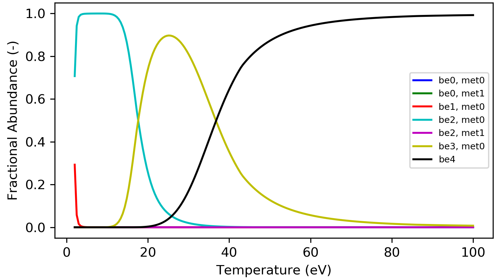
The time independent solution as a function of electron temperature is shown below.
 1temp = np.linspace(2,100,200) #temp grid
 2ion = ionization_balance(fils, metas, temp, dens, keep_species_data = False)
 3ion.populate_ion_matrix()
 4ion.solve_time_independent()
 5
 6
 7fig, ax1 = plt.subplots(1,1,figsize=(16/3.,9/3.),dpi=300)
 8fig.subplots_adjust(bottom=0.15,top=0.99,left=0.11,right=0.99)
 9
10ax1.plot(temp,ion.data['pops_ss'][0,0,:,1],label='be0, met0',color='b')
11
12ax1.plot(temp,ion.data['pops_ss'][1,0,:,1],label='be0, met1',color='g')
13
14ax1.plot(temp,ion.data['pops_ss'][2,0,:,1],label='be1, met0',color='r')
15
16ax1.plot(temp,ion.data['pops_ss'][3,0,:,1],label='be2, met0',color='c')
17
18ax1.plot(temp,ion.data['pops_ss'][4,0,:,1],label='be2, met1',color='m')
19
20ax1.plot(temp,ion.data['pops_ss'][5,0,:,1],label='be3, met0',color='y')
21
22ax1.plot(temp,ion.data['pops_ss'][6,0,:,1],label='be4',color='k')
23
24ax1.legend(fontsize='x-small')
25
26ax1.set_xlabel('Temperature (eV)')
27ax1.set_ylabel('Fractional Abundance (-)')